In this tutorial, we'll learn how to use grid visualization with different indicator scales. Currently, there are two ways of using a grid in CleverMaps:
-
connecting your
geometryPointdataset usingh3Griddatasets with grid geometries generated on the fly -
mapping your
geometryPointdataset using AreaMapper and importing a grid data dimension with vector tiles
This tutorial covers both cases. It's up to you if you want to learn only one of them or both.
What you'll create
We will add a grid visualization and some more indicator scales.
|
|
|
|
|
|
|
|
|
|
Using H3 grid
CleverMaps natively supports visualization using the H3 grid spatial index developed by Uber. This hierarchical spatial index consists of several resolutions of grid cells which cover the whole Earth, and are related to each other (similar to lower and higher administrative units). The differences between this approach and using AreaMapper and data dimension are:
-
The geometries are not in vector tile format, but are generated on the fly by the application frontend
-
There is no need for pre-computed DWH datasets in the project - H3 grids have generated cell names
-
The grid can be used for any location on Earth (in any resolution)
The usage is also much simpler - to use the H3 grid visualization we need to:
-
add some
h3Griddatasets (each for one resolution) -
add these datasets to the
ref.h3Geometriesarray of thegeometryPointdataset we want to visualize
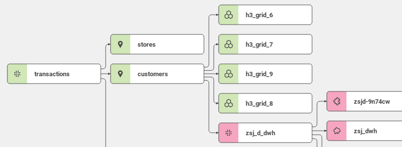
So, let's add these 4 h3Grid datasets:
|
Resolution 6 |
Resolution 7 |
Resolution 8 |
Resolution 9 |
h3_grid_6.json
|
h3_grid_7.json
|
h3_grid_8.json
|
h3_grid_9.json
|
Use addMetadata to add these datasets. Now add the h3Geometries reference to the customers dataset:
Customers dataset excerpt
   ...
        "ref": {
            "type": "dwh",
            "subtype": "geometryPoint",
            "h3Geometries": [
                "h3_grid_6",
                "h3_grid_7",
                "h3_grid_8",
                "h3_grid_9"
            ],
            "visualizations": [
                {
                    "type": "dotmap"
                },
   ...
And use pushProject to push the changes. You can review the references to the h3Grid datasets in the data model.
Now you can skip right to Tutorial 8: AreaMapper and grid visualization#Grid visualization, or explore the second way - AreaMapper and data dimension.
Advanced Tips for H3 grids
-
Is H3 grid insufficient in performance? The use case described here is a basic one. It's possible to use dataset with materialized H3 grid ID columns which makes the responses up to 2-3x times faster.
-
If you need connect multiple fact tables, it is necessary to use materialized H3 grid dimension with materialized DWH datasets. In the example bellow, the dataset
cz_uc4_grid_res9_dwhcan be connected with multiple fact datasets from the left side:
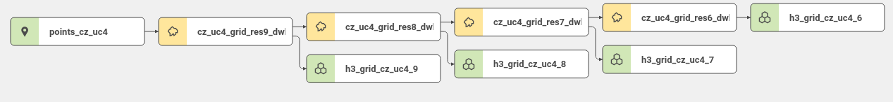
Contact us at support@clevermaps.io for more information about H3 grids.
Using AreaMapper and data dimension
Running AreaMapper
CleverMaps AreaMapper is one of our . AreaMapper computes geometric intersection between points and polygons (areas, grids) and then adds IDs of polygons to the points table if an intersection exists.
It can be run in Docker or at Keboola. We will use Docker because not everyone has a Keboola account and it can be run locally.
You can get Docker here. Select Docker Desktop and download the installation file according to your platform.
Then use the following command to get the AreaMapper image:
docker pull clevermaps/areamapper:latest
We will create an empty directory on our local drive (e.g. /home/user/CleverMaps/AreaMapper) and copy the customers.csv file from the first tutorial into the folder.
Now, we will create a configuration file for AreaMapper. There are two possible ways of running AreaMapper:
-
using polygons CSV on your local drive
-
using polygons CSV prepared and hosted by us
The difference is - when using local CSV, you can use any CSV you want. When using the hosted CSV, the file has to be hosted by us first. For more info, contact us at info@clevermaps.io. The current list of hosted dimensions can be found here.
The CSV we will use in this tutorial is already hosted. In case you want to try the "local" way, or just have a look at the CSV, you can download it here.
|
Hosted CSV |
Local CSV |
config-hosted.json
|
config-local.json
|
We will run AreaMapper using the following command. Please note that you have to modify the paths according to your system.
user@host:/home/user/CleverMaps/AreaMapper$ sudo docker run -t -v /home/user/CleverMaps/AreaMapper:/workdir clevermaps/areamapper:latest --config /workdir/config-hosted.json

Importing /workdir/customers.csv to temp database...
Importing /workdir/cz_grid_res9_wkt.csv to temp database...
Creating geometry on points table...
Creating geometry on polygons table...
Creating spatial index on points table...
Creating spatial index on polygon table...
Calculating intersection...
Area mapping was successfully finished.
Copy the output file you specified in the JSON config (customers_mapped.csv) to your project dump /data folder and rename it to customers.csv to overwrite the older customers CSV.
Importing the grid dimension
Let's import the grid data dimension using the importProject command.
tomas.schmidl@secure.clevermaps.io/project:k5t8mf2a80tay2ng/dump:2020-06-23_17-48-00$ importProject --project nbutdscdghhg25v4 --datasets
Importing project nbutdscdghhg25v4...
Here, we omit a significant amount of the importProject command output for the sake of readability.
Import finished!
Source project: nbutdscdghhg25v4 (can-dim-grid-cz-uber)
Destination project: k5t8mf2a80tay2ng (First project)
Imported datasets: 9
Imported metadata objects: 0
Imported CSV files: 4

To view detailed imported content, use status command.
Now you can make changes, or import another project.
When you're done, use addMetadata command to add the metadata to the project.
To push the data to the project, use pushProject command.
Add the imported files using addMetadata and pushProject.
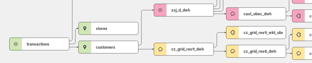
Now we have to edit the customers dataset. AreaMapper added one column to the end of the CSV file - hex_id. We have to add this property to the end of our dataset. Its foreign key will point to the lowest grid dataset - cz_grid_res9_dwh.
Customers dataset excerpt
  ...
        {
            "name": "lng",
            "title": "Address longitude",
            "column": "lng",
            "type": "longitude",
            "filterable": false
        },
        {
            "foreignKey": "cz_grid_res9_dwh",
            "name": "hex_id",
            "title": "Hex grid ID",
            "column": "hex_id",
            "type": "string",
            "filterable": false
        }
    ],
  ...
Take a look at the data model to see that the customers and cz_grid_res9_dwh are joined.
Grid visualization
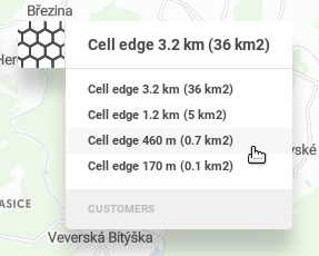
Enter the Business overview view, and select the new granularity from the granularity drop-down menu.
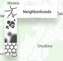
Now, we have a new visualization available - a grid.
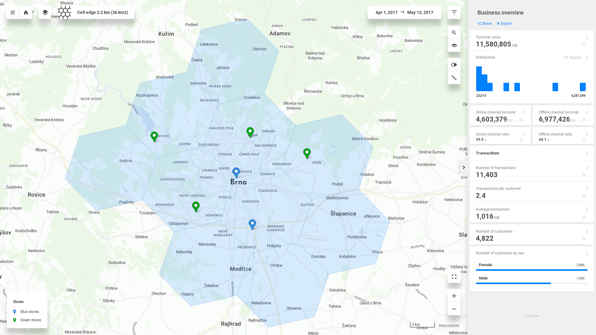
Alternatively, select one of the lower levels to get to a bigger detail.
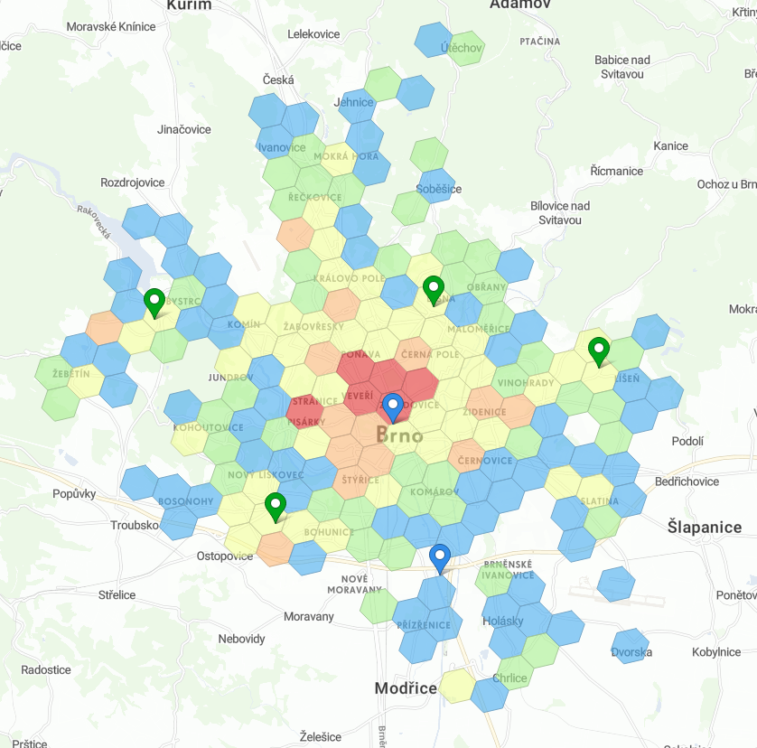
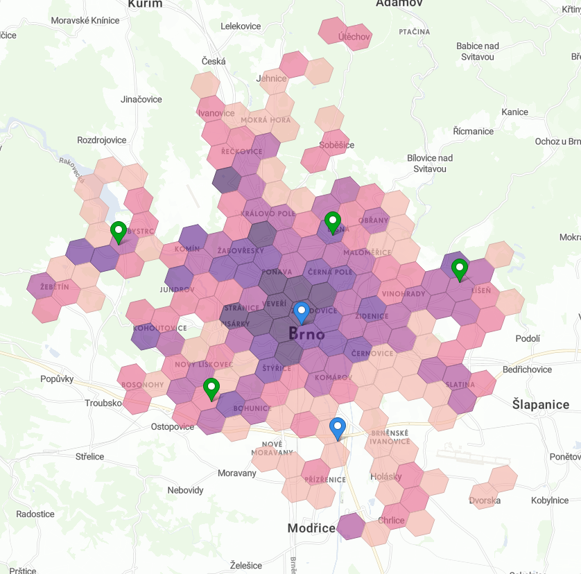
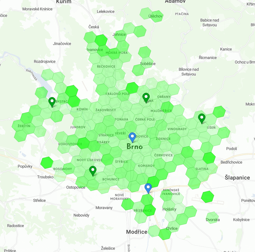
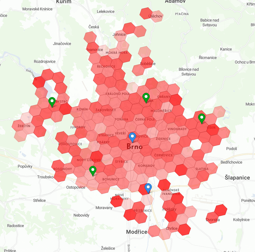
Indicator scales
Let's take a look at more indicator scales. So far we've used only the standard (blue) scale.
To try some of them, set the following scales for these indicators:
-
for
online_turnover_indicator, setcontent.scaleto "heatmap" -
for
offline_turnover_indicator, setcontent.scaleto "magma" -
for
online_ratio_indicator, setcontent.scaleto "positive" -
for
offline_ratio_indicator, setcontent.scaleto "negative"
Use pushProject to push the indicators and enter the view. Select the grid visualization, select one of the lower levels (e.g. "Cell edge 460 m") and click "Visualize" on the "Online channel turnover" indicator.
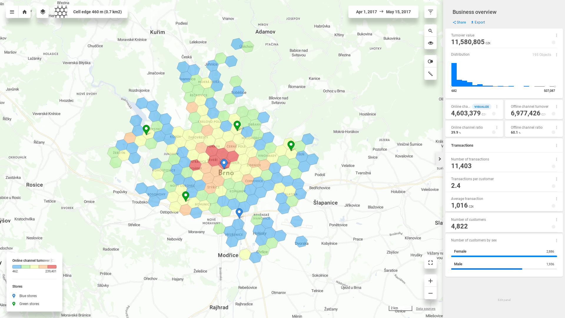
But indicators offer way more scales. Feel free to explore them and use them in your projects!
That's it! The last part of CleverMaps tutorial is a bit more technical and focused on Shell project management.